Results
Results of Finite Element Analysis
Figure 26 depicts the stress distribution and displacement. According to this data, the maximum displacement was 2.176mm and the maximum Von-Mises stress was 27.84MPa. This confirms our theory that the simulation will have smaller results for these values since the model contained a solid structure rather than stranding.
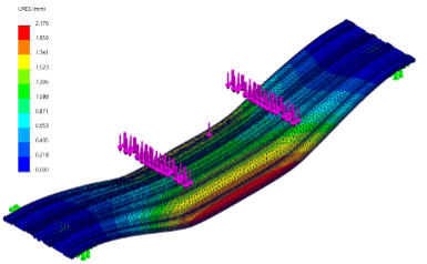
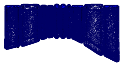
Furthermore, the cable did not experience linear bending due to the asymmetrical layout of the wires. This can be seen in Figure 27, where the sides deform more than the center. As a result, the value for maximum displacement is not an accurate representation of the strain experienced by the cable due to the load. A better alternative is to replace the load with a predetermined displacement in the simulation and determine the stress from there. However, the simulation software ran into many issues, so we used the average displacement from the first study instead.
Results of Four-Point Bend Test
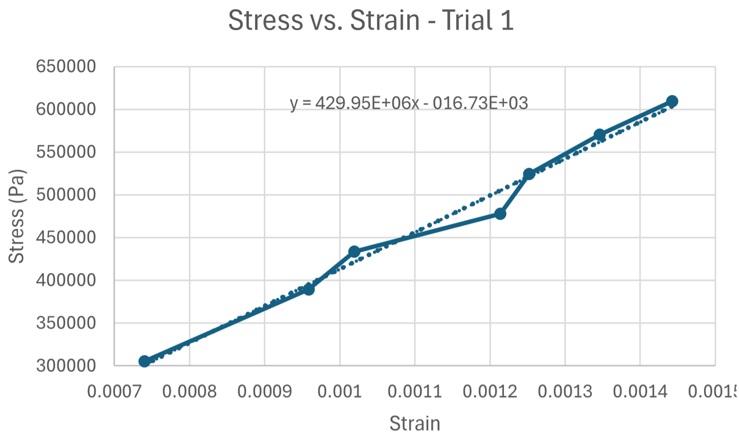
Trial 1

Trial 2

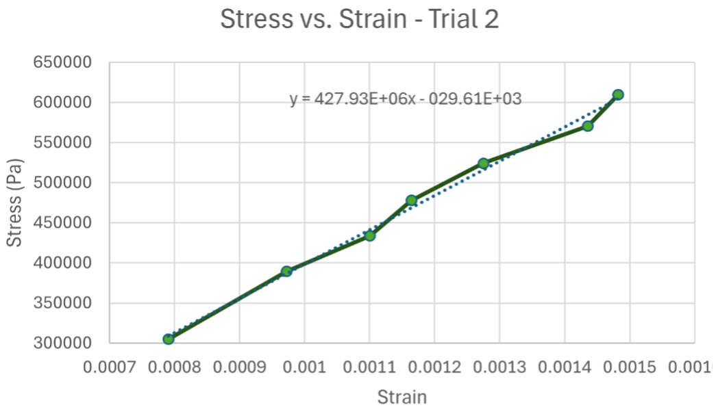
From these 2 trials, we were able to obtain the following for the Bending Modulus:

Using this average value for the Bending Modulus, we are able to approximate the Bending Stiffness by multiplying it by the 2nd Moment of Inertia. The only issue with this is that the cable has an extremely complicated cross-section, meaning that we will have to approximate it as a rectangle. When doing this, we obtain an Approximate Moment of Inertia (I):
I = 608 mm4
Now we can use the value to obtain the Bending Stiffness (EI):
EI = 428.94 N/mm2 * 608 mm4 = 2.605 × 10⁵ Nmm2
This value will be used to compare our results using the different methods (Static & Dynamic).
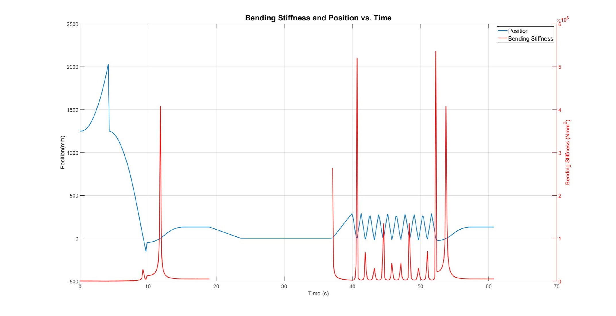
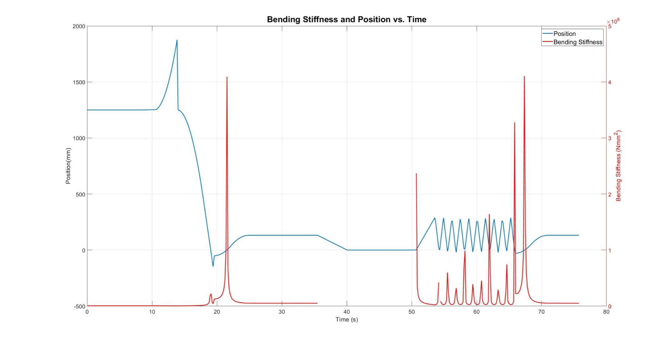
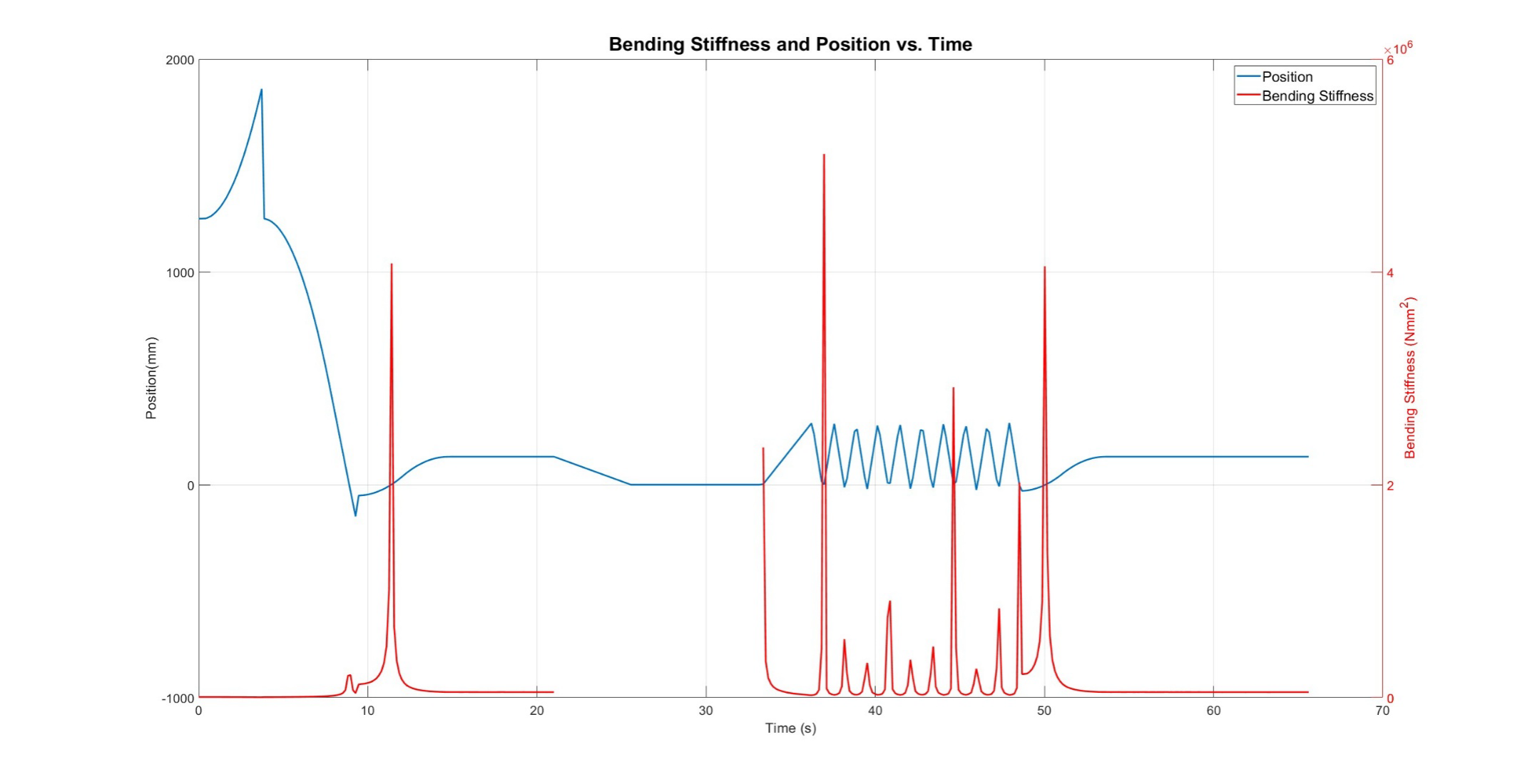
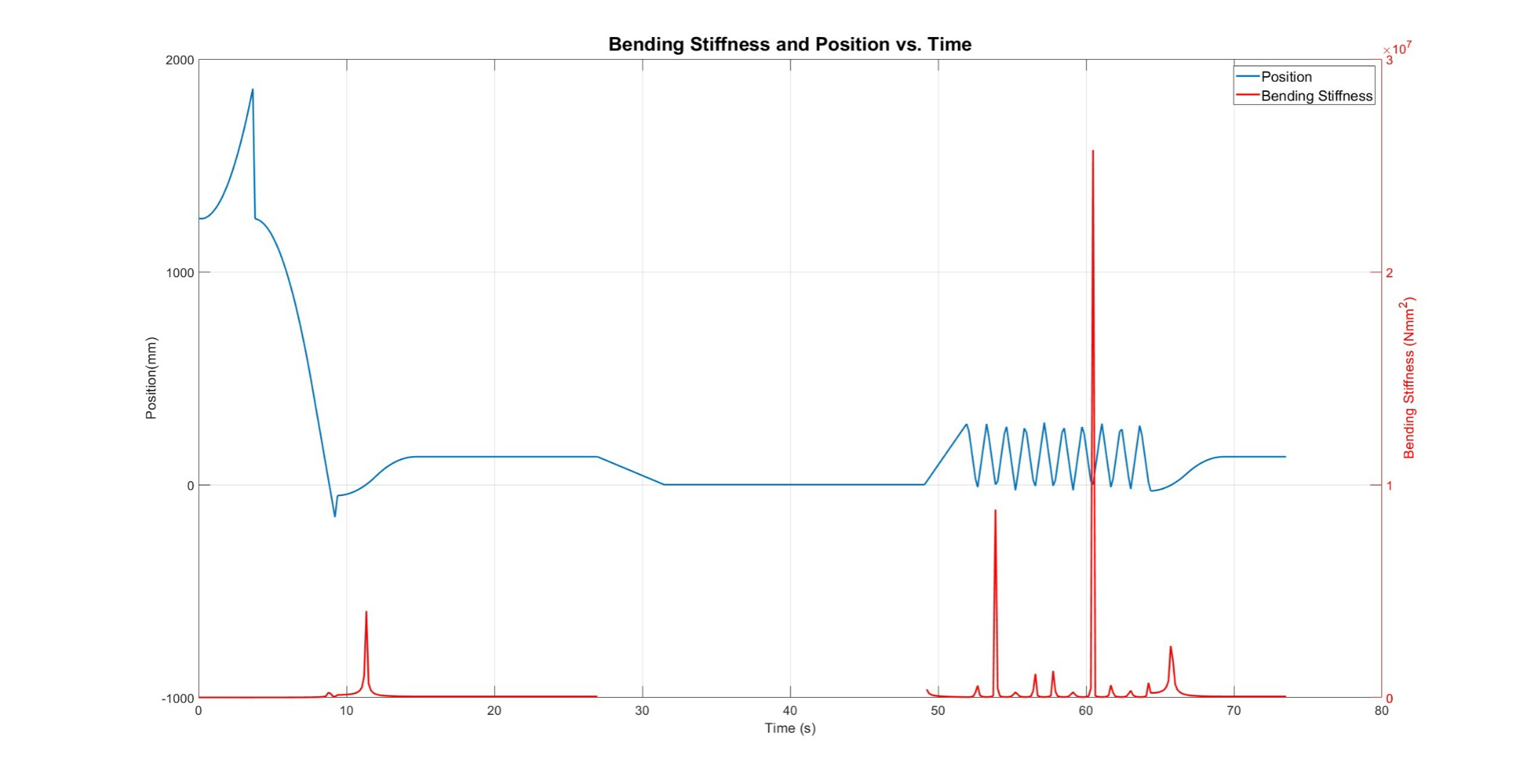
Results of the Dynamic Test
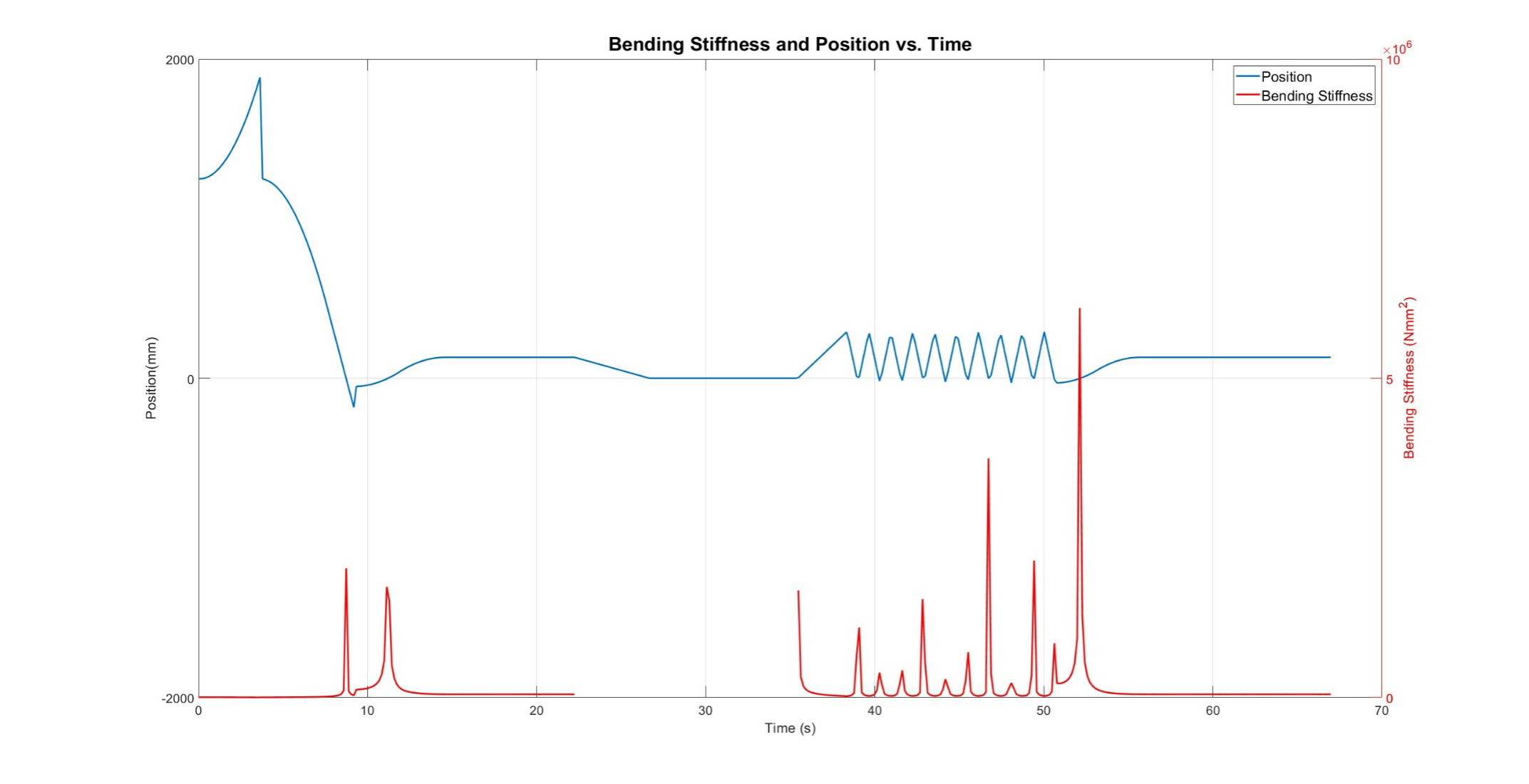
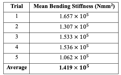
Using our test fixture, we were able to obtain an approximate value for the Bending Stiffness of the ASML cable. We ran 5 different tests and obtained the Bending Stiffness for each one, from which we took the average to obtain our final result. In the following graphs, you will find the results for the Bending Stiffness versus Time. Also important to note is that for our follow-up calculations based on the data in these graphs, we have decided not to use every single Bending Stiffness data point to obtain the average result. This is because the cable was observed to be sagging when it reached the extremes of the travel distance. From this observation, we decided to exclude datapoints after a certain position (190mm). Another observation we made after obtaining the data was that there are points in time when the cable crosses the zero position during the loops. Because of the way our final equation for the Bending Stiffness is set up, we were getting extremely high peaks of datapoints for the Bending Stiffness. To combat this, we decided to exclude any data where the cable would go past the zero position in the negative direction and only decided to observe the positive region (x > 0.5mm).
Trial 1
Trial 2
Trial 3
Trial 4
Trial 5