Introduction

Background

In 1984, Advanced Semiconductor Materials Lithography emerged from a joint venture between Philips and ASM International. Known today as ASML, the company has enjoyed immense success, expanding its operations to offices worldwide and employing over 44,000 employees [1]. From humble beginnings, the company has established itself as one of the world’s leading chip-making equipment manufacturers. Without ASML’s machines, the most recognizable names in tech, such as Intel or TSMC, would not continue their operations and manufacture the millions of microchips needed to keep life moving forward [2].

Although ASML has diversified its product lineup with metrology equipment, it is deeply rooted in lithography systems [3]. Lithography is typically the first stage of silicon wafer processing. Formally known as photolithography, this process projects UV light through a mask containing the desired patterns onto wafers covered in thin photoresist films. The induced chemical process transfers patterns carried by light onto the wafer and allows for further steps such as deposition or etching [4].

Most innovations within lithography systems involve speed, volume, and above all else, resolution. While ASML offers industry-standard deep ultraviolet (DUV) systems (enabling feature sizes of 38nm) [5], their latest innovation, extreme ultraviolet (EUV) systems (enabling feature sizes of 8nm) [6], looks to uphold Moore’s Law for as long as possible. The contributing factor for such increased resolutions is the fourteen times shorter wavelengths EUV systems can output [5].

Taking their ‘EXE’ system to the peak of innovation required optimizing an additional aspect: speed. Single wafers may have to be patterned hundreds of times before being diced into chips, a potentially lengthy process. Maximizing the output of their machines, measured in wafers per hour, ASML developed a reticle that accelerates linearly at 32g; for perspective, a car experiencing this acceleration would go from 0 to 60 mph in less than a tenth of a second [7]. Completing this action requires a significant amount of power and vacuum; currently, a robust FCC array with integrated hose lines is fixed onto the top of the optic bay and looped down to the magnetic reticle stage. This cable undergoes a continuous yet erratic rolling bend while the machine operates.

Project Description

Our team was tasked with determining the bending stiffness of the cables supplied in collaboration with analysis engineers from ASML. Data collected from our tests would further the company’s modeling capabilities and analysis. Such data is fundamental in diagnosing flaws and verifying future improvements. Meeting the strict accuracy requirements for projects of such magnitude required acquiring and comparing data from static and dynamic tests. In turn, the team worked on supplying testing equipment for both cases.

Apart from the industry-specific aspect of this project, it serves as our senior design capstone project. The academic goal of the class was to experience every aspect of the product development cycle that competent engineers must adhere to. Only being given an overall goal by ASML, the team had to develop novel concepts, evaluate feasibility, generate and validate designs against desired outcomes, manufacture prototypes, and run tests before presenting the final product. Facing the complex challenges that arise at the intersection of engineering analysis and product development provided a rite of passage for our team.

Motivation

To maintain market dominance and uphold its reputation, ASML must ensure its machines run as intended for as long as possible. In the semiconductor industry, downtime (specifically unplanned downtime) for any machine results in significant losses and frustration. Business Korea reported that in 2020, a Samsung factory lost over 43 million dollars because of a 30-minute power outage [8]. Apart from total failure, downtime may occur from the malfunction of a single component. ASML engineers suspect the robust nature of their power cables in combination with extreme accelerations may lead to early degradation, compromising their effectiveness.

Integrated circuits must be manufactured with nanometer precision; therefore, all nanofabrication facilities are cleanrooms. These specialized facilities constantly filter air through HEPA filters to minimize the risk of particles contaminating the wafer surface. Federal standards designate clean rooms by class, each determined by the particle concentration per cubic foot of air [9]. To minimize contamination and comply with the cleanroom environment, ASML’s machines operate under vacuum. Unfortunately, the necessary conditions for producing chips are at risk if these cables rapidly degrade; determining the bending stiffness of such cables provides invaluable data for amending the issue. Rectifying potential problems before they cause a rift between customer and supplier will sustain the powerful relationships propelling ASML forward.

Literature Search

The main benefit of a literature search is optimizing time and resources; gaining a deeper understanding of the problem and possible solutions minimizes potential errors. Before generating concepts and drafting designs, our team investigated four main topics: cable characteristics, material properties, static test methodology, and existing dynamic test equipment. Gauging common cable characteristics and their impact on properties such as bending stiffness against the cables supplied by ASML laid the groundwork for our intuition of the magnitude of forces we may be dealing with. Pairing classroom knowledge with external sources relating material properties with stress, strain, and force was key in directing us towards the equations we would need to apply when manipulating future data. Likewise, evaluating patents for existing static and dynamic wire testing equipment aided our decision-making process when designing our innovative solution.

General information

Manufacturers enhance power cable designs by considering various factors, weighing each advantage and trade-off against the intended application. In ASML's case, flexibility is a critical limiting factor. Thus, examining the conductive core, insulating material, and overall construction is essential. There are two types of conductive cores: stranded and solid. Stranded wires are more expensive; however, they offer greater flexibility and longer flex lives in motion applications [10].

PVC and PTFE are the most commonly used insulation materials. PTFE, also known as Teflon, is favored in high-performance applications due to its exceptional thermal, chemical, and electrical stability. Although less durable, PVC is widely used for household applications because of its low cost and superior flexibility [11]. The round cable construction offers beneficial properties that improve reliability against mechanical stress, yet FCCs provide greater flexibility [12]. The FCC, with a stranded core and PTFE insulation supplied for testing, incorporates thoughtful design considerations, although questions remain about whether the supplier optimized it for the expected conditions.

Bending stiffness (EI) measures a cable’s resistance to bending, which is crucial for its performance under cyclic loading. According to the CIGRE B1 Technical Brochure, Reference 862, this stiffness property is defined by the relationship between the bending moment and curvature, often exhibiting non-linear behavior [13]. Specifically, as the curvature applied to a cable increases, the stiffness increases until plastic deformation occurs. Besides a cable's geometry, key factors influencing the stiffness include magnitude, temperature, bending rate, and amplitude [13]. An accurate assessment of overall bending stiffness is essential, providing critical insights into a cable's durability under operational stress.

The ANSI/NEMA WC53/ICEA T-27-581-2020 standard further supports this characterization by outlining standard physical tests for insulated cables, especially in Section 4 – Physical Methods [14]. While this standard does not specifically measure bending stiffness or modulus values, it includes methods for assessing mechanical durability and deformation resistance. Sections 4.2 (Cold Bend) and 4.4 (Flexibility Test for Interlocked Armor) evaluate the integrity of cables when subjected to flexing and bending conditions [14]. These qualitative tests confirm whether a cable can endure repeated or extreme bending without fracturing or cracking.

Section 4.3 (Heat Deformation) also details tests that expose cables to compressive loads at elevated temperatures, demonstrating the extent of permanent deformation that occurs under thermal-mechanical stress [14]. While these tests do not provide direct measurements of stiffness or modulus, they offer insights into how material stiffness evolves in thermally active environments. Section 4.11 (Tensile Strength, Stress, and Elongation Tests) presents a standardized procedure for stretching cable components to the point of failure. By collecting stress-strain data throughout these tests, Young’s modulus (E) can be derived using Hooke’s Law in the linear elastic region [14].

Overall, these physical methods create a consistent framework for indirectly assessing the mechanical resilience and deformation resistance of cables, serving as a foundation for our quantitative approaches.

Static Analysis - 4 Point Bending

Bending stiffness is commonly evaluated using three-point and four-point bending tests. The three-point bending method applies a central load between two supports, creating a bending moment with a non-uniform stress distribution. While this method is suitable for initial analysis, its accuracy is limited due to uneven force application.

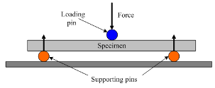
We will conduct a four-point bending test following ASTM D6272 to accurately quantify the FCC's bending stiffness. This test setup will establish a region with a constant bending moment and zero shear between the inner loading points, creating ideal conditions for flexural characterization.

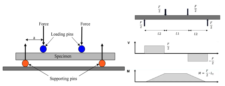
Following ASTM conventions, where the load span equals half the support span, we will calculate the maximum outer fiber stress and the midspan strain. These calculations will allow us to determine Young’s modulus using Hooke’s Law [15]:

With Young’s modulus known, we will be able to calculate the bending stiffness:

This approach will enable us to derive bending stiffness based on fundamental beam mechanics while adhering to ASTM’s elastic limit guidelines, which allow for strains of up to 5%. Unlike simplified flexural stiffness formulas that rely solely on load and deflection, this method will rigorously capture the material-specific elastic response and geometry.

Although TAPPI/ANSI T 836 utilizes a moment-based stiffness equation tailored for corrugated materials, its procedures reinforce our assumptions: small-deflection conditions, delayed deflection readings, and careful span and clamp control are critical for ensuring repeatability and accuracy [15][16]. The standard emphasizes allowable strain ranges and deflection precision, further supporting the validity of our method across composite and flexible cable-like structures.

In summary, this analytical framework, rooted in ASTM D6272 and supported by TAPPI T 836, provides a consistent and validated approach for determining flexural stiffness in the cable system. The EI values obtained serve as essential input for both static deflection modeling and dynamic system response analysis in the project's later phases.

Dynamic Analysis – Semicircular Cable Assembly

Just like with the 4-point static test, this study aims to obtain the effective bending stiffness of the cable. The difference between the dynamic and static analyses is that the cable is in a semicircular curved state and is experiencing a displacement on one of the ends. This dynamic configuration was inspired by standard cable fatigue tests commonly utilized in industrial validation. Among these tests, the C-Track and Tick-Tock tests are frequently employed to simulate repetitive bending in motion systems. The C-Track test subjects cables to guided bending through carriers, while the Tick-Tock test uses a pendulum-style motion to bend the cable around a fixed mandrel repeatedly [17]. While both methods are designed to assess fatigue life, they do not provide quantitative insights into cable stiffness.

Our team was particularly influenced by the Rolling Bend Test, which eliminates fixed-radius supports and allows for unsupported, continuous flexing. This method lets the cable bend freely and naturally distribute strain along its length [18]. This approach closely resembles the conditions our semicircular test assembly would be designed to replicate. By modifying this protocol into a tool for measuring mechanical stiffness, we transformed a fatigue-oriented test into a tool for measuring mechanical stiffness, a critical parameter for modeling deformation in high-precision environments.

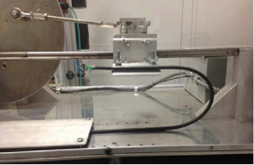
In this case the cable was configured into a fixed-fixed semicircular arch with a known radius of 75mm. Knowing this setup, an experimental approach combined with theoretical analysis based on established structural mechanics principles was adopted.

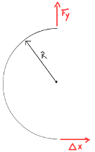
The analytical foundation for this method was sourced from Roark's Formulas for Stress and Strain (7th Edition), Chapter 9, Table 9.3, titled "Reaction and deformation formulas for circular arches." This table provides comprehensive solutions for various arch configurations and loading conditions. The experimental setup corresponds to Case 5: "Left end fixed, right end fixed" within this table.

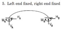
Roark’s provides a set of general deformation equations for this case, which relate the displacements (d_HA, d_VA) and rotation (c_A) at one end of the arch (denoted as end A) to the corresponding reaction forces (H_A, V_A) and moment (M_A) at that same end. These equations incorporate stiffness/compliance coefficients (B_ij), which are functions of the arch’s geometry (specifically the half-angle ψ) and factors k₁, k₂ that account for hoop stress and shear deformation [19]. The general form of these equations is:

Here, LF_H, LF_V, and LF_M are terms that depend on any externally applied loads.

It's important to note that Roark’s standard diagrams for arches orient the baseline (the line connecting the supports) horizontally. In our physical setup, the U-shape of the arch opens to the right, meaning the line connecting the two fixed clamps is vertical. This requires a careful mapping of our physical displacements and forces to Roark’s terminology. The specific conditions substituted into Roark’s general equations for end A were:

• Arch Geometry:
  The arch is a semicircle, so its half-angle ψ = π/2 radians (90°)
• Applied Displacement at End A (e.g., the “bottom” moving clamp in your setup):
  The motor applies a physical horizontal displacement, Δx_physical. Due to our setup’s orientation (U-shape opening to the right, line of supports is vertical), this physical horizontal displacement is perpendicular to Roark’s arch baseline. Thus, it corresponds to Roark’s vertical displacement at end A: d_VA = Δx_physical
• Other Constraints at End A:
  • The physical displacement along the line of supports (Roark’s horizontal displacement) is zero: d_HA = 0
  • The rotation at the fixed end A is zero: c_A = 0
• Measured Reaction Force:
  We are measuring the physical vertical force, F_y,physical, which in this orientation is along Roark’s arch baseline. This is being measured at the other fixed end (end B), it corresponds to Roark’s horizontal reaction force at end B: H_B = F_y,physical (The derivation will solve for H_A, and then H_B = −H_A due to overall horizontal equilibrium).
• External Loads:
  No external loads are applied during this specific test, so the load terms LF_H = 0, LF_V = 0, LF_M = 0
• Simplification:
  For this analysis, the minor effects of hoop stress and shear deformation were neglected, meaning Roark’s correction factors k₁ and k₂ were approximated as 1.

These specific conditions, when substituted into Roark’s general system of three deformation equations for Case 5 (along with the B_ij coefficients for ψ = π/2), allow the system to be solved algebraically for the reactions at end A (H_A, V_A, M_A). From H_A, we find H_B (= F_y,physical) in terms of the applied d_VA (= Δx_physical), the radius R, and the bending stiffness EI_eff [19].

With these conditions (physical horizontal displacement Δx_physical corresponding to Roark’s d_VA at end A, other displacements/rotations at A being zero, and no external loads), the specific values for the B_ij coefficients for a semicircle (ψ = π/2, k₁ = k₂ = 1) were determined as (e.g., B_HH = π/2, B_HV = 2, etc.). Substituting these coefficients and the specific displacement conditions (d_HA = 0, d_VA = Δx_physical, c_A = 0) into the general deformation equations transformed them into a solvable system of three linear algebraic equations with H_A, V_A, and M_A as the unknown reactions at end A.

This system was then solved algebraically for the horizontal reaction force H_A (which corresponds to the negative of the physical vertical force F_y,physical measured at the other fixed end B, i.e., H_A = −H_B = −F_y,physical, or directly to F_y,physical if measured at end A with appropriate sign convention) in terms of the applied physical horizontal displacement Δx_physical (which is d_VA in Roark’s frame), the radius R, and the bending stiffness EI_eff. The algebraic solution of the system of equations yielded the following relationship for the magnitude of the horizontal reaction force |H_A| (and thus |H_B|):

This equation was then rearranged to solve for the effective bending stiffness:

Replacing |H_B| with our physically measured vertical force |F_y,physical| and |Δx_physical| with our physically applied horizontal displacement, the formula remains:

The dimensionless constant K = (72 − π²)/16 is approximately 3.883. Thus, the final working formula used to determine the bending stiffness from the experimental data, based on Roark’s formulas, is: